Temperature Autoregression — a leak-free evaluation walkthrough

This notebook is a self-contained walkthrough of the ``swedish-temperatures:ar`` problem in emflow: a least-squares autoregressive (AR) model that forecasts hourly air temperature one hour ahead for the SMHI station Stockholm-Observatoriekullen A.

The model is trained on all data before 2026 and evaluated on 2026.

The point of this notebook: to make it unmistakably clear that the evaluation has no data leakage. Every claim below is backed by a runnable assert — if the evaluation leaked, a cell would fail.

All data is bundled inside the emflow package, so this notebook runs top-to-bottom offline — no network access required.

# On Colab, uncomment to install the package (the dataset ships with it):
# !pip install emflow

import numpy as np
import pandas as pd
import matplotlib.pyplot as plt

import emflow as ef
from emflow.examples.swedish_temperatures.predictor import ARPredictor
from emflow.problems.objective import MeanSquaredError

1. Load the problem

emflow problems are loaded by name. Each returns a (dataset, environment, objective) triple. The dataset (a single Parquet file) is bundled in the package and read via importlib.resources — nothing is downloaded.

ef.list_problems()

['gefcom2014-solar:simple',
 'heftcom2024:baseline',
 'solar-battery',
 'swedish-temperatures:ar']

dataset, env, obj = ef.load_problem("swedish-temperatures:ar")

print(dataset.description)
print()
temps = dataset.data["temperatures"]
series = temps.iloc[:, 0]                      # the Stockholm temperature series
print("Station   :", temps.columns[0])
print("Full range:", series.index.min(), "->", series.index.max())
print("Objective :", obj.name)

Hourly air temperature (°C) from SMHI station Stockholm-Observatoriekullen A (id 98230). Benchmark for 1-step-ahead autoregressive forecasting: train < 2026, evaluate on 2026.

Station   : ('98230', 'Stockholm-Observatoriekullen A')
Full range: 2016-06-02 08:00:00+00:00 -> 2026-06-02 08:00:00+00:00
Objective : MeanAbsoluteError

2. Explore the data

Ten years of hourly temperatures. The red line marks TEST_START (2026-01-01): everything to its left is available for training, everything to its right is the evaluation period.

Note the honest caveat: SMHI’s corrected-archive (quality-controlled) data ends ~3 months before “now”, so the actual observations stop on 2026-03-01. The later 2026 rows exist but are NaN and are simply skipped when scoring.

fig, ax = plt.subplots(figsize=(11, 3))
ax.plot(series.index, series.values, lw=0.3)
ax.axvline(env.test_start, color="red", ls="--", lw=1.5, label="TEST_START (2026-01-01)")
ax.set_title("Hourly air temperature — Stockholm-Observatoriekullen A")
ax.set_ylabel("°C"); ax.legend(loc="lower left")
plt.tight_layout(); plt.show()

print("Last real observation:", series.last_valid_index())

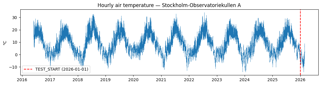
Last real observation: 2026-03-01 06:00:00+00:00

3. The evaluation contract — what the model is (and isn’t) allowed to see

The environment enforces the train/test boundary:

• ``env.reset()`` returns the training data (initial_data["target"], timestamps before TEST_START) plus a forecast input.

• ``env.step()`` returns the test actuals — and only after we’ve made our predictions.

So the targets we are scored against are handed back last. The model never sees them while fitting or predicting.

initial_data, forecast_input = env.reset()
train = initial_data["target"]

print("Train rows        :", f"{len(train):,}")
print("Last training hour:", train.index.max())
print("TEST_START        :", env.test_start)

# The model is fit strictly on the past:
assert train.index.max() < env.test_start
print("\nassert train.index.max() < TEST_START  ->  OK")

Train rows        : 83,992
Last training hour: 2025-12-31 23:00:00+00:00
TEST_START        : 2026-01-01 00:00:00+00:00

assert train.index.max() < TEST_START  ->  OK

4. The autoregressive model

ARPredictor fits an ordinary-least-squares AR model

\[\hat{y}_t = c + \sum_i w_i\, y_{t-\ell_i}, \qquad \ell \in \{1,\dots,24\}\cup\{168\}\]

i.e. the previous 24 hours plus the same hour one week earlier, with an intercept. It is plain numpy.linalg.lstsq — no scaler or normalizer is fit on the data, so no global/test statistic can sneak in.

model = ARPredictor()           # lags = [1..24, 168]
model.train(train)              # <-- fit on TRAIN ONLY

col = train.columns[0]
intercept, weights = model.coefs[col]
print("lags          :", model.lags)
print("n parameters  :", len(weights) + 1, "(intercept + lags)")
print("intercept     :", round(intercept, 4))
print("lag-1 weight  :", round(float(weights[model.lags.index(1)]), 4))
print("largest |w| at: lag", model.lags[int(np.abs(weights).argmax())],
      "(temperature is highly persistent)")

lags          : [1, 2, 3, 4, 5, 6, 7, 8, 9, 10, 11, 12, 13, 14, 15, 16, 17, 18, 19, 20, 21, 22, 23, 24, 168]
n parameters  : 26 (intercept + lags)
intercept     : 0.0115
lag-1 weight  : 1.2349
largest |w| at: lag 1 (temperature is highly persistent)

5. Forecast and evaluate on 2026

We predict, then call env.step() to reveal the actuals, then score. We compare the AR model against two naive baselines on the same test hours:

• Persistence: \(\hat{y}_t = y_{t-1}\)

• Seasonal-naive (24h): \(\hat{y}_t = y_{t-24}\)

preds = model.predict(forecast_input)          # 1-step-ahead forecasts
_, test_target, done = env.step()              # actuals revealed now

y    = test_target.iloc[:, 0]
yhat = preds.iloc[:, 0].reindex(y.index)
persistence = series.shift(1).reindex(y.index)
seasonal    = series.shift(24).reindex(y.index)

mse = MeanSquaredError()
def score(p):
    return obj.calculate(y, p), mse.calculate(y, p, squared=False)   # MAE, RMSE

results = pd.DataFrame(
    {"AR (lags 1-24+168)": score(yhat),
     "Persistence (t-1)":  score(persistence),
     "Seasonal naive (t-24)": score(seasonal)},
    index=["MAE (°C)", "RMSE (°C)"],
).T.round(3)

n_eval = int(y.reindex(yhat.index).notna().sum())
print(f"Evaluated on {n_eval:,} non-missing test hours (2026)")
results

Evaluated on 1,423 non-missing test hours (2026)

	MAE (°C)	RMSE (°C)
AR (lags 1-24+168)	0.289	0.399
Persistence (t-1)	0.313	0.455
Seasonal naive (t-24)	2.261	2.937

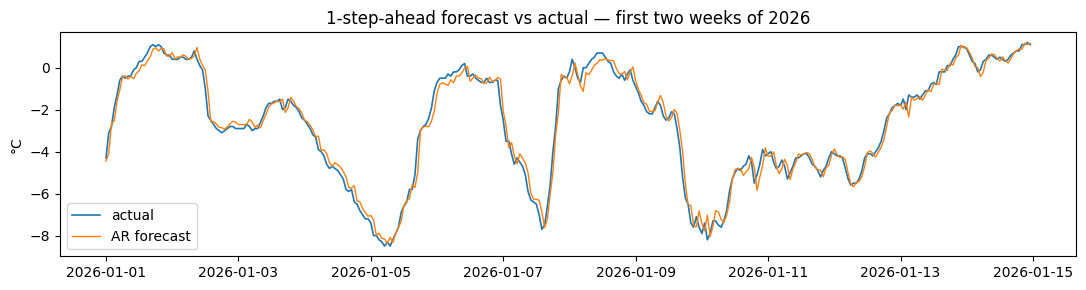
win = slice("2026-01-01", "2026-01-14")
fig, ax = plt.subplots(figsize=(11, 3))
ax.plot(y.loc[win].index, y.loc[win].values, label="actual", lw=1.2)
ax.plot(yhat.loc[win].index, yhat.loc[win].values, label="AR forecast", lw=1.0)
ax.set_title("1-step-ahead forecast vs actual — first two weeks of 2026")
ax.set_ylabel("°C"); ax.legend()
plt.tight_layout(); plt.show()

6. No data leakage — demonstrated

It can look suspicious that env.reset() hands the predictor the full series (including the test period). Below we prove that this is purely a vectorization convenience and cannot leak: every forecast \(\hat{y}_t\) depends only on observations strictly before \(t\).

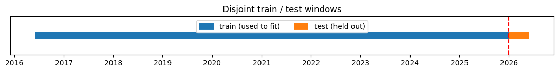
(a) The train and test windows are disjoint

train_idx, test_idx = train.index, y.index
assert train_idx.max() < env.test_start <= test_idx.min()
assert len(train_idx.intersection(test_idx)) == 0
print("train:", train_idx.min(), "->", train_idx.max())
print("test :", test_idx.min(), "->", test_idx.max())
print("overlap:", len(train_idx.intersection(test_idx)), "hours")

fig, ax = plt.subplots(figsize=(11, 1.5))
ax.hlines(1, train_idx.min(), train_idx.max(), color="C0", lw=10, label="train (used to fit)")
ax.hlines(1, test_idx.min(),  test_idx.max(),  color="C1", lw=10, label="test (held out)")
ax.axvline(env.test_start, color="red", ls="--")
ax.set_yticks([]); ax.legend(loc="upper center", ncol=2); ax.set_title("Disjoint train / test windows")
plt.tight_layout(); plt.show()

train: 2016-06-02 08:00:00+00:00 -> 2025-12-31 23:00:00+00:00
test : 2026-01-01 00:00:00+00:00 -> 2026-06-02 08:00:00+00:00
overlap: 0 hours

(b) The model was fit on the past only

model.train(train) received data ending at the last training hour below — months before any test timestamp.

print("model.train() input ended at:", train.index.max())
print("first test timestamp        :", test_idx.min())
assert train.index.max() < test_idx.min()
print("OK — fit data strictly precedes the evaluation period.")

model.train() input ended at: 2025-12-31 23:00:00+00:00
first test timestamp        : 2026-01-01 00:00:00+00:00
OK — fit data strictly precedes the evaluation period.

(c) Each forecast uses strictly past lags

To predict the very first test hour, the model only references earlier timestamps (the previous 24 hours and 168h earlier) — all of which fall in the training period.

t0 = test_idx.min()
lag_times = [t0 - pd.Timedelta(hours=L) for L in model.lags]
assert all(lt < t0 for lt in lag_times)
print("To predict", t0, "the model uses (all strictly earlier):")
print("  ", [str(lag_times[0]), str(lag_times[1]), "...", str(lag_times[-1])])
print("  all < t and all in the training period:", all(lt < env.test_start for lt in lag_times))

To predict 2026-01-01 00:00:00+00:00 the model uses (all strictly earlier):
   ['2025-12-31 23:00:00+00:00', '2025-12-31 22:00:00+00:00', '...', '2025-12-25 00:00:00+00:00']
  all < t and all in the training period: True

(d) The whole supervised dataset in one picture

Here is the most direct way to see there is no leakage. Each 1-step-ahead prediction is one sample: its inputs are the lag timestamps \(\{t-1,\dots,t-24,\,t-168\}\) and its output is the target time \(t\). We loop over target hours straddling the train/test boundary, collect each sample, and plot the times: x-axis = sample, y-axis = time, with one colour for inputs and one for outputs.

Read the chart two ways:

• For every sample (every x), all input points lie below the output point — the model only ever looks back in time. (Leakage would be an input above its output; that never happens.)

• The green region holds samples whose target is before TEST_START — these (input → output) pairs are exactly the rows model.train() was fit on. The red region holds samples predicted but never trained on (the 2026 test set).

# Build one (output_time, input_times) sample per prediction, around the boundary.
window = pd.Timedelta(hours=100)
targets = series.index[(series.index >= env.test_start - window) &
                       (series.index <= env.test_start + window)]

samples = []                                   # (output_time, input_times)
for t in targets:
    input_times = pd.DatetimeIndex([t - pd.Timedelta(hours=L) for L in model.lags])
    if series.reindex(input_times).notna().all() and pd.notna(series.loc[t]):
        samples.append((t, input_times))       # a genuine design-matrix row

# The ridiculously-easy leakage check: every input is strictly before its output.
assert all(input_times.max() < t for t, input_times in samples)
n_train = sum(t < env.test_start for t, _ in samples)
print(f"{len(samples)} samples ({n_train} train, {len(samples) - n_train} test) — "
      "for EVERY one, all inputs precede the output. ✓")

201 samples (100 train, 101 test) — for EVERY one, all inputs precede the output. ✓

naive = lambda ts: pd.DatetimeIndex(ts).tz_convert(None)   # drop tz for plotting only

fig, ax = plt.subplots(figsize=(12, 6))
for x, (t, input_times) in enumerate(samples):
    ax.scatter([x] * len(input_times), naive(input_times), s=8, color="tab:blue")
    ax.scatter([x], naive([t]), s=22, color="tab:orange", zorder=3)

# Train vs test shown via background regions (keeps just two point colours).
ax.axvspan(-0.5, n_train - 0.5, color="tab:green", alpha=0.07)
ax.axvspan(n_train - 0.5, len(samples) - 0.5, color="tab:red", alpha=0.07)
ax.axvline(n_train - 0.5, color="black", ls=":", lw=1)
ax.axhline(pd.Timestamp(env.test_start).tz_convert(None), color="red", ls="--", lw=1)

ymax = ax.get_ylim()[1]
ax.text(n_train * 0.5, ymax, "TRAIN\n(model.train fit on these)",
        ha="center", va="top", color="green", fontsize=9)
ax.text((n_train + len(samples)) * 0.5, ymax, "TEST\n(predicted, never trained on)",
        ha="center", va="top", color="firebrick", fontsize=9)

from matplotlib.lines import Line2D
ax.legend(handles=[
    Line2D([0], [0], marker="o", ls="", color="tab:blue", label="input (lag) times"),
    Line2D([0], [0], marker="o", ls="", color="tab:orange", label="output (target) time"),
], loc="lower right")
ax.set_xlabel("sample index (ordered by target time)")
ax.set_ylabel("time")
ax.set_title("Every prediction's inputs lie strictly below (before) its output\n"
             "red dashed line = TEST_START")
plt.tight_layout(); plt.show()

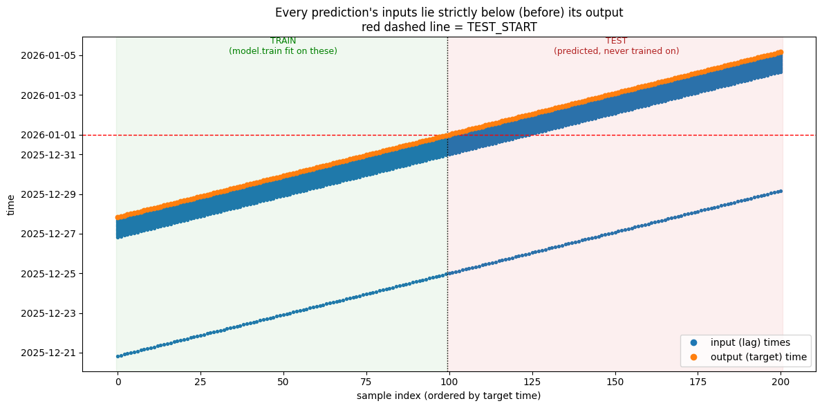
Notice that the test samples (red region) have inputs dipping below the TEST_START line: they legitimately use already-observed history as lags. That is allowed — what matters is that no input ever sits above its own output.

(e) Causality proof: hide the present and future, predictions don’t change

For a set of test timestamps \(t^\*\), we recompute the forecast from a copy of the series in which every value at :math:`t ge t^*` is deleted (set to NaN). If a prediction secretly used present/future information, it would change. It does not: the maximum difference is exactly 0.

full_pred = model.predict(forecast_input).iloc[:, 0]

def predict_with_future_hidden(cutoff):
    masked = forecast_input.copy()
    masked.loc[masked.index >= cutoff] = np.nan     # hide present + future
    return model.predict(masked).iloc[:, 0]

# Sample test hours that actually have a forecast (most of Mar-Jun 2026 is NaN),
# always including the very first test hour. Sample by position to keep tz info.
rng = np.random.default_rng(0)
predictable = full_pred.dropna().index
predictable = predictable[predictable >= env.test_start]
pos = rng.choice(len(predictable), size=min(50, len(predictable)), replace=False)
sample = [test_idx.min()] + [predictable[p] for p in pos]

max_diff, n_checked = 0.0, 0
for t in sample:
    a = full_pred.loc[t]
    b = predict_with_future_hidden(t).loc[t]
    if np.isnan(a) and np.isnan(b):
        continue                                    # lag genuinely missing in both
    max_diff = max(max_diff, abs(float(a) - float(b)))
    n_checked += 1

print(f"checked {n_checked} test hours")
print("max |Δ| between full-series and future-hidden forecasts:", max_diff)
assert max_diff == 0.0
print("✓ Every forecast depends only on strictly past observations — no leakage.")

checked 51 test hours
max |Δ| between full-series and future-hidden forecasts: 0.0
✓ Every forecast depends only on strictly past observations — no leakage.

(f) Corrupting every test actual leaves early forecasts untouched

As a final illustration: add large random noise to all test-period values and re-predict the first test hour. Because its lags lie entirely in the (untouched) training period, the forecast is byte-for-byte identical.

noise = pd.DataFrame(0.0, index=forecast_input.index, columns=forecast_input.columns)
m = forecast_input.index >= env.test_start
noise.loc[m] = rng.normal(0, 10, size=(int(m.sum()), forecast_input.shape[1]))
corrupted = forecast_input + noise

orig = model.predict(forecast_input).iloc[:, 0].loc[t0]
corr = model.predict(corrupted).iloc[:, 0].loc[t0]
print("first test-hour forecast — original :", round(float(orig), 6))
print("first test-hour forecast — corrupted:", round(float(corr), 6))
assert orig == corr
print("✓ Corrupting all test actuals does not change the first test forecast.")

first test-hour forecast — original : -4.449448
first test-hour forecast — corrupted: -4.449448
✓ Corrupting all test actuals does not change the first test forecast.

7. Recap & next steps

• The split is disjoint, the model is fit on the past only, there is no preprocessing leak, and each 1-step-ahead forecast provably uses strictly past lags — verified above with hard asserts.

• The AR model comfortably beats persistence and seasonal-naive baselines.

Ideas to extend this:

• All 15 stations — ARPredictor already loops over columns; drop the single-station selection in the problem to forecast the whole network.

• Multi-step horizons — roll the AR forward recursively and watch error grow.

• Fresher 2026 data — top up past the 2026-03-01 archive cutoff with SMHI’s latest-months period (note: that tail is provisional, not yet quality-corrected).